"But his delight is in the law of the LORD; and in his law doth he meditate day and night."
-->

| Where the quail is whistling betwixt the woods and the wheat-lot; | ||||
| Where the bat flies in the Seventh-month eve—where the great gold-bug drops through the dark; | ||||
| Where flails keep time on the barn floor; | ||||
| Leaves of Grass 33 lines 731-33 |

Chess:
| Laplace Transform | |
The Laplace transform is an integral transform perhaps second only to the Fourier transform in its utility in solving physical problems. The Laplace transform is particularly useful in solving linear ordinary differential equations such as those arising in the analysis of electronic circuits.
The (unilateral) Laplace transform  (not to be confused with the Lie derivative, also commonly denoted
  ) is defined by
(not to be confused with the Lie derivative, also commonly denoted ) is defined by =int_0^inftyf(t)e^(-st)dt,](https://mathworld.wolfram.com/images/equations/LaplaceTransform/NumberedEquation1.gif) |
(1)
|
where  is defined for
  =0" border="0" width="27" height="14"> (Abramowitz and Stegun 1972). The unilateral Laplace transform is almost always what is meant by "the" Laplace transform, although a bilateral Laplace transform is sometimes also defined as
is defined for =0" border="0" width="27" height="14"> (Abramowitz and Stegun 1972). The unilateral Laplace transform is almost always what is meant by "the" Laplace transform, although a bilateral Laplace transform is sometimes also defined as =int_(-infty)^inftyf(t)e^(-st)dt](https://mathworld.wolfram.com/images/equations/LaplaceTransform/NumberedEquation2.gif) |
(2)
|
(Oppenheim et al. 1997). The unilateral Laplace transform ](https://mathworld.wolfram.com/images/equations/LaplaceTransform/Inline5.gif) is implemented in Mathematica as LaplaceTransform[f[t], t, s].
is implemented in Mathematica as LaplaceTransform[f[t], t, s].
is implemented in Mathematica as LaplaceTransform[f[t], t, s].
The inverse Laplace transform is known as the Bromwich integral, sometimes known as the Fourier-Mellin integral (see also the related Duhamel's convolution principle).
A table of several important one-sided Laplace transforms is given below.
 | ](https://mathworld.wolfram.com/images/equations/LaplaceTransform/Inline7.gif) | conditions |
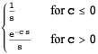
| 1 |  | |
 |  | |
 |  |  =0" border="0" width="57" height="14"> =0" border="0" width="57" height="14"> |
 |  |  -1" border="0" width="62" height="14"> -1" border="0" width="62" height="14"> |
 |  | |
 |  |  |
 |  |  |I[omega]|" border="0" width="54" height="14"> |I[omega]|" border="0" width="54" height="14"> |
 |  |  |R[omega]|" border="0" width="59" height="14"> |R[omega]|" border="0" width="59" height="14"> |
 |  |  |I[omega]|" border="0" width="54" height="14"> |I[omega]|" border="0" width="54" height="14"> |
 |  |  a+|I[b]|" border="0" width="73" height="14"> a+|I[b]|" border="0" width="73" height="14"> |
 |  |  |
 |  | |
 |  0" border="0" width="111" height="59"> 0" border="0" width="111" height="59"> | |
 |  | |
 |  |  =0" border="0" width="57" height="14"> =0" border="0" width="57" height="14"> |
In the above table,  is the zeroth-order Bessel function of the first kind,
  is the delta function, and
  is the Heaviside step function.
is the zeroth-order Bessel function of the first kind, is the delta function, and is the Heaviside step function.
The Laplace transform has many important properties. The Laplace transform existence theorem states that, if  is piecewise continuous on every finite interval in
  satisfying
is piecewise continuous on every finite interval in satisfying
(3)
|
for all  , then
 ](https://mathworld.wolfram.com/images/equations/LaplaceTransform/Inline52.gif) exists for all
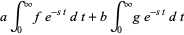
exists for all  a" border="0" width="29" height="14">. The Laplace transform is also unique, in the sense that, given two functions
  and
and  with the same transform so that
, then exists for all a" border="0" width="29" height="14">. The Laplace transform is also unique, in the sense that, given two functions and with the same transform so that =L_t[F_2(t)](s)=f(s),](https://mathworld.wolfram.com/images/equations/LaplaceTransform/NumberedEquation4.gif) |
(4)
|
then Lerch's theorem guarantees that the integral
 |
(5)
|
vanishes for all  0" border="0" width="30" height="14"> for a null function defined by
0" border="0" width="30" height="14"> for a null function defined by  |
(6)
|
The Laplace transform is linear since
![L_t[af(t)+bg(t)]](https://mathworld.wolfram.com/images/equations/LaplaceTransform/Inline57.gif) |  | ![int_0^infty[af(t)+bg(t)]e^(-st)dt](https://mathworld.wolfram.com/images/equations/LaplaceTransform/Inline59.gif) |
(7)
|
 |  |  |
(8)
|
 |  | ![aL_t[f(t)]+bL_t[g(t)].](https://mathworld.wolfram.com/images/equations/LaplaceTransform/Inline65.gif) |
(9)
|
The Laplace transform of a convolution is given by
![L_t[f(t)*g(t)]=L_t[f(t)]L_t[g(t)] L_t^(-1)[FG]=L_t^(-1)[F]*L_t^(-1)[G].](https://mathworld.wolfram.com/images/equations/LaplaceTransform/NumberedEquation7.gif) |
(10)
|
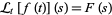
 be continuously differentiable
  times in
  . If , then
 =s^nL_t[f(t)]-s^(n-1)f(0)-s^(n-2)f^'(0)-...-f^((n-1))(0).](https://mathworld.wolfram.com/images/equations/LaplaceTransform/NumberedEquation8.gif) |
(11)
|
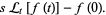
This can be proved by integration by parts,
](https://mathworld.wolfram.com/images/equations/LaplaceTransform/Inline70.gif) |  | 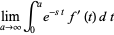 infty)int_0^ae^(-st)f^'(t)dt" border="0" width="112" height="35"> infty)int_0^ae^(-st)f^'(t)dt" border="0" width="112" height="35"> |
(12)
|
 |  | 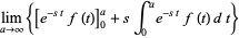 infty){[e^(-st)f(t)]_0^a+sint_0^ae^(-st)f(t)dt}" border="0" width="209" height="35"> infty){[e^(-st)f(t)]_0^a+sint_0^ae^(-st)f(t)dt}" border="0" width="209" height="35"> |
(13)
|
 |  |
(14)
| |
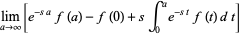 |  |  infty)[e^(-sa)f(a)-f(0)+sint_0^ae^(-st)f(t)dt]" border="0" width="235" height="35"> infty)[e^(-sa)f(a)-f(0)+sint_0^ae^(-st)f(t)dt]" border="0" width="235" height="35"> |
(15)
|
 |  |
(16)
| |
 |  | ![sL_t[f(t)]-f(0).](https://mathworld.wolfram.com/images/equations/LaplaceTransform/Inline85.gif) |
(17)
|
Continuing for higher-order derivatives then gives
=s^2L_t[f(t)](s)-sf(0)-f^'(0).](https://mathworld.wolfram.com/images/equations/LaplaceTransform/NumberedEquation9.gif) |
(18)
|
This property can be used to transform differential equations into algebraic equations, a procedure known as the Heaviside calculus, which can then be inverse transformed to obtain the solution. For example, applying the Laplace transform to the equation
 |
(19)
|
gives
-sf(0)-f^'(0)}+a_1{sL_t[f(t)](s)-f(0)}+a_0L_t[f(t)](s)=0](https://mathworld.wolfram.com/images/equations/LaplaceTransform/NumberedEquation11.gif) |
(20)
|
(s^2+a_1s+a_0)-sf(0)-f^'(0)-a_1f(0)=0,](https://mathworld.wolfram.com/images/equations/LaplaceTransform/NumberedEquation12.gif) |
(21)
|
which can be rearranged to
=(sf(0)+f^'(0)+a_1f(0))/(s^2+a_1s+a_0).](https://mathworld.wolfram.com/images/equations/LaplaceTransform/NumberedEquation13.gif) |
(22)
|
If this equation can be inverse Laplace transformed, then the original differential equation is solved.
The Laplace transform satisfied a number of useful properties. Consider exponentiation. If =F(s)](https://mathworld.wolfram.com/images/equations/LaplaceTransform/Inline86.gif) for
for  alpha" border="0" width="30" height="14"> (i.e.,
  is the Laplace transform of
  ), then
 =F(s-a)](https://mathworld.wolfram.com/images/equations/LaplaceTransform/Inline90.gif) for
for  a+alpha" border="0" width="52" height="14">. This follows from
for alpha" border="0" width="30" height="14"> (i.e., is the Laplace transform of ), then for a+alpha" border="0" width="52" height="14">. This follows from  | 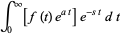 |  |
(23)
|
 |  | ![int_0^infty[f(t)e^(at)]e^(-st)dt](https://mathworld.wolfram.com/images/equations/LaplaceTransform/Inline97.gif) |
(24)
|
 |  | .](https://mathworld.wolfram.com/images/equations/LaplaceTransform/Inline100.gif) |
(25)
|
The Laplace transform also has nice properties when applied to integrals of functions. If  is piecewise continuous and , then
is piecewise continuous and , then ![L_t[int_0^tf(t^')dt^']=1/sL_t[f(t)](s).](https://mathworld.wolfram.com/images/equations/LaplaceTransform/NumberedEquation14.gif) |
(26)
|
REFERENCES:
Abramowitz, M. and Stegun, I. A. (Eds.). "Laplace Transforms." Ch. 29 in Handbook of Mathematical Functions with Formulas, Graphs, and Mathematical Tables, 9th printing. New York: Dover, pp. 1019-1030, 1972.
Arfken, G. Mathematical Methods for Physicists, 3rd ed. Orlando, FL: Academic Press, pp. 824-863, 1985.
Churchill, R. V. Operational Mathematics. New York: McGraw-Hill, 1958.
Doetsch, G. Introduction to the Theory and Application of the Laplace Transformation. Berlin: Springer-Verlag, 1974.
Franklin, P. An Introduction to Fourier Methods and the Laplace Transformation. New York: Dover, 1958.
Graf, U. Applied Laplace Transforms and z-Transforms for Scientists and Engineers: A Computational Approach using a Mathematica Package. Basel, Switzerland: Birkhäuser, 2004.
Jaeger, J. C. and Newstead, G. H. An Introduction to the Laplace Transformation with Engineering Applications. London: Methuen, 1949.
Henrici, P. Applied and Computational Complex Analysis, Vol. 2: Special Functions, Integral Transforms, Asymptotics, Continued Fractions. New York: Wiley, pp. 322-350, 1991.
Krantz, S. G. "The Laplace Transform." §15.3 in Handbook of Complex Variables. Boston, MA: Birkhäuser, pp. 212-214, 1999.
Morse, P. M. and Feshbach, H. Methods of Theoretical Physics, Part I. New York: McGraw-Hill, pp. 467-469, 1953.
Oberhettinger, F. Tables of Laplace Transforms. New York: Springer-Verlag, 1973.
Oppenheim, A. V.; Willsky, A. S.; and Nawab, S. H. Signals and Systems, 2nd ed. Upper Saddle River, NJ: Prentice-Hall, 1997.
Prudnikov, A. P.; Brychkov, Yu. A.; and Marichev, O. I. Integrals and Series, Vol. 4: Direct Laplace Transforms. New York: Gordon and Breach, 1992.
Prudnikov, A. P.; Brychkov, Yu. A.; and Marichev, O. I. Integrals and Series, Vol. 5: Inverse Laplace Transforms. New York: Gordon and Breach, 1992.
Spiegel, M. R. Theory and Problems of Laplace Transforms. New York: McGraw-Hill, 1965.
Weisstein, E. W. "Books about Laplace Transforms." http://www.ericweisstein.com/encyclopedias/books/LaplaceTransforms.html.
Widder, D. V. The Laplace Transform. Princeton, NJ: Princeton University Press, 1941.
Zwillinger, D. (Ed.). CRC Standard Mathematical Tables and Formulae. Boca Raton, FL: CRC Press, pp. 231 and 543, 1995.
CITE THIS AS:
Weisstein, Eric W. "Laplace Transform." From MathWorld--A Wolfram Web Resource. http://mathworld.wolfram.com/LaplaceTransform.html


No comments:
Post a Comment